Gradient boosting is a machine learning technique for regression and
classification problems which produces a prediction model in the form of an
ensemble of weak prediciton models, typically descision trees. The model is
built in stages like other boosting methods where each stage fits the residual
of the previous stage.
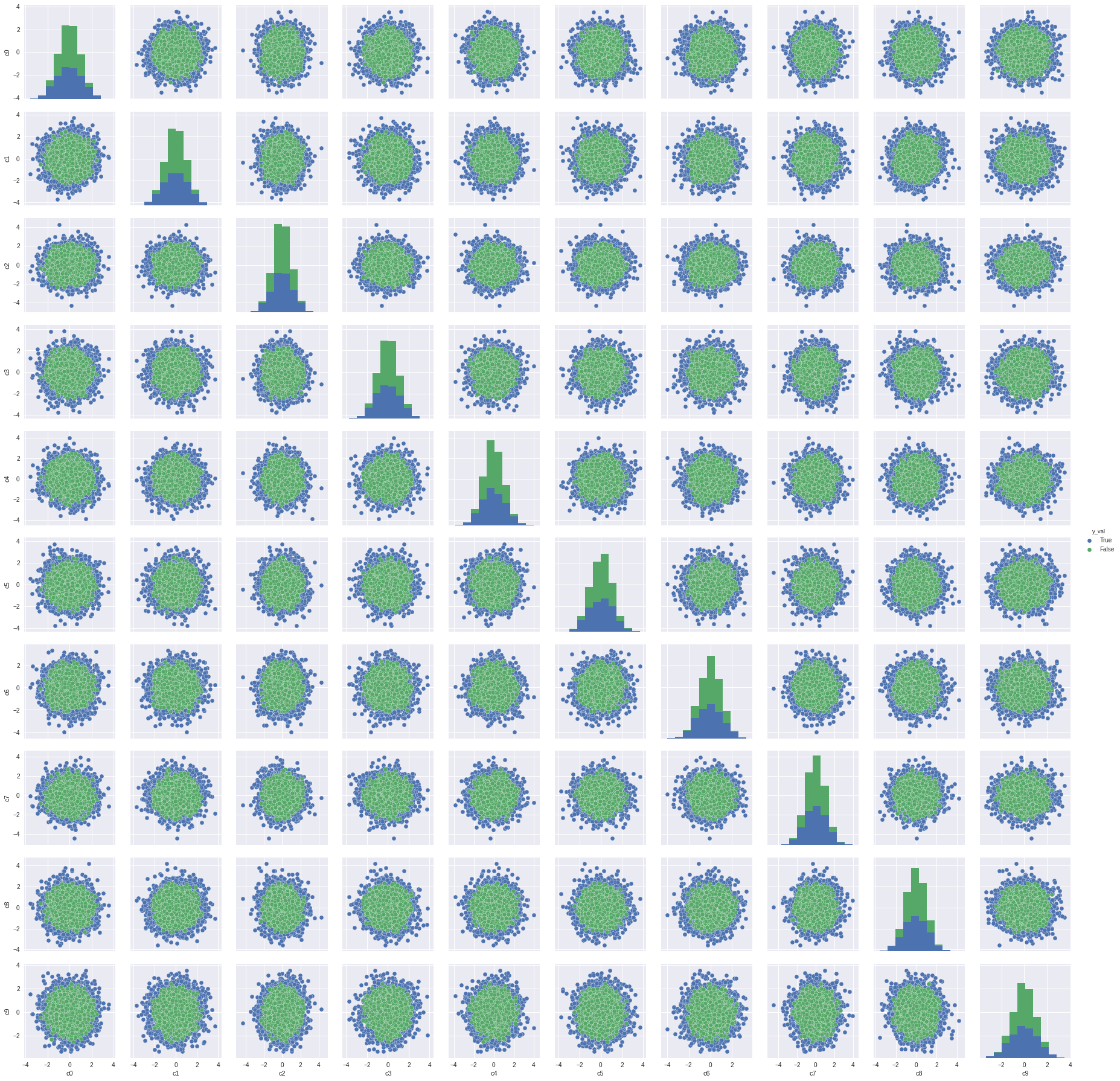
We first create a synthetic dataset from Hastie et al 2009, example 10.2.
# 5000 rows, 10 columns of X values with each column having# a mean 0 and standard deviation 1# Approximately half the y values are -1 and the other half are 1fromsklearn.datasetsimport make_hastie_10_2
X, y = make_hastie_10_2(n_samples=5000)
The table below shows the mean and standard deviations of the 10 columns
1
2
3
4
5
6
7
8
9
10
mean
-0.01
0.01
-0.02
0.01
-0.03
0.03
-0.01
0.00
0.00
0.00
stdev
1.00
1.01
1.00
1.00
1.01
1.01
1.00
1.01
1.00
1.01
There is significant overlap of the y values as shown by the green and blue
dots.
Pair wise plot
Applying the gradient boosting classifier we can estimate the
accuracy.
# split the data into training and test samples
X_train, X_test, y_train, y_test = train_test_split(X, y)
# fit estimator
est = GradientBoostingClassifier(n_estimators=200, max_depth=3)
est.fit(X_train, y_train)
# predict class labels
pred = est.predict(X_test)
# score on test data (accuracy)
acc = est.score(X_test, y_test)
print('ACC: %.4f'% acc)
The importance of each of the 10 features is given below and all features are
important.
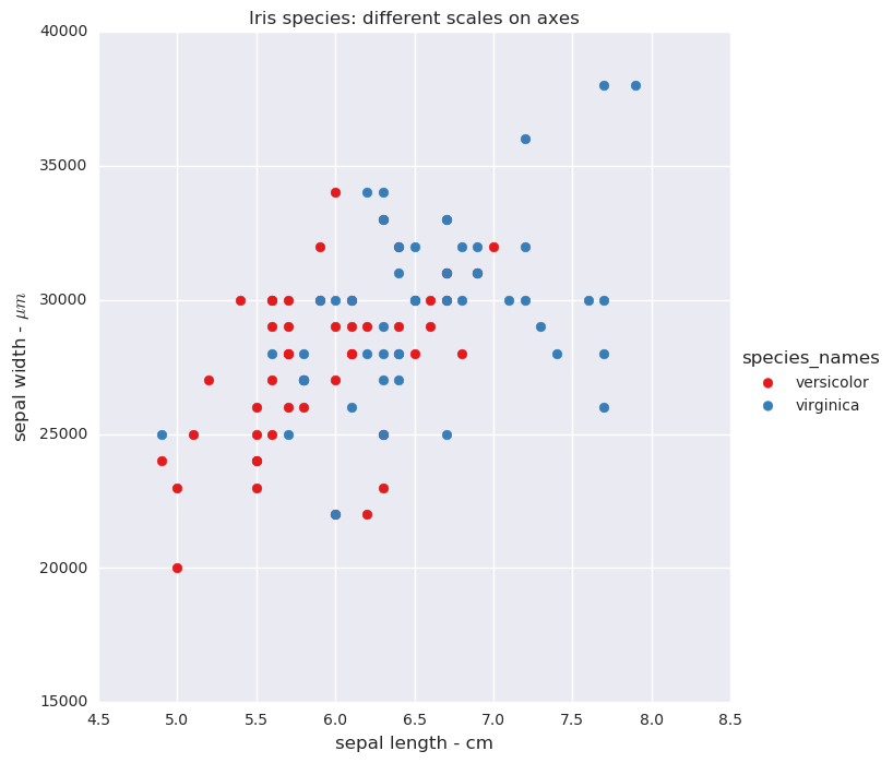
Some machine learning algorithms in the sklearn library are affected by data measured using different scales. For example if one measure is in centimeters (one hundreth of a meter) and another is in micrometers (one millionth of a meter) the results may not be optimal.
Sklearn has scaling functions in the preprocessing module
Load the Iris dataset. It has three kinds of Irises with each Iris species stored in 50 consecutive rows. Loading the second and third Iris species stored from row 50 and above create a subset of the data.
Display the two species versicolor and virginica with two axis: sepal length and sepal width. The sepal length is in centimeters and the sepal width is in micrometers.
Iris species: different scales on x and y axes
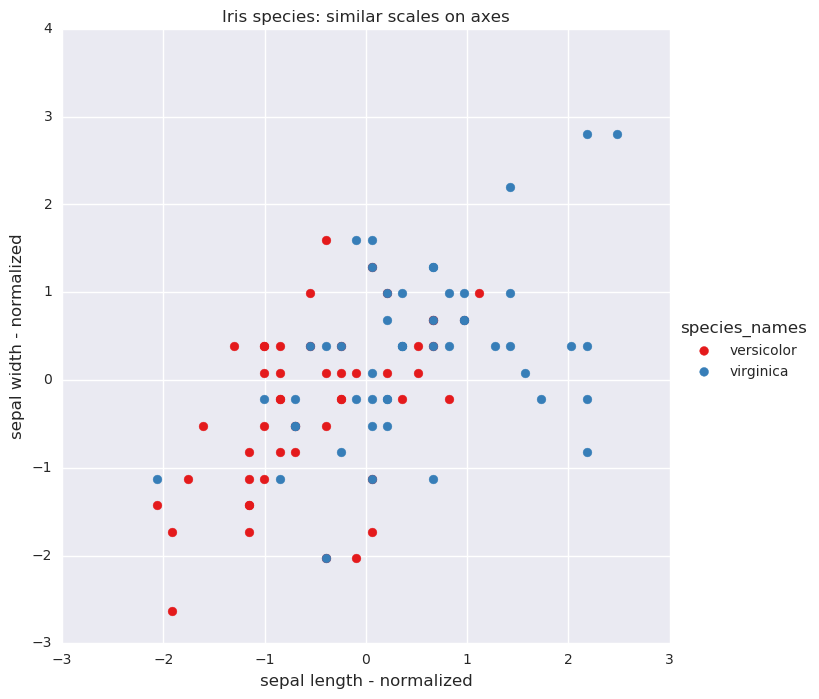
Using the scale function in sklearn the measures are converted to have a mean of zero and variance of one.
measure
sepal length
sepal width
species
count
1.000000e+02
1.000000e+02
100.0000
mean
3.288481e-15
4.496403e-17
1.500000
stdev
1.005038e+00
1.005038e+00
0.502519
Iris species: normalized axes
Using logistic regression and a decision tree classifier with the original data
and normalized data the results are in the table below.
classifier
accuracy
precision
recall
Logistic regression: different scales
0.56
0.578947
0.44
Logistic regression: normalized data
0.75
0.745098
0.76
Decision tree: different scales
0.88
0.816667
0.98
Decision tree: normalized data
0.88
0.816667
0.98
The logistic regression method improves when using normalized data however the
decision tree method does equally well with the original data and the
normalized data.
Cross-validation is a technique used to assess how a statistical analysis will generalize to an independent data set.
When creating a predictive model, the model is trained using a dataset called the training dataset. The accuracy of the trained model is then tested on another unknown dataset called the testing dataset. The process is called cross-validation.
Scikit learn makes it easy to use multiple methods for cross validation. A basic approach is called k-fold cross validation. The dataset is split into k smaller sets, where 1 of the sets is used to validate the model while the remaining are used to train the model. The peformance measures reported by the k-fold cross-validations are the average of the values computed by choosing a different set for the cross-validation and using the remaining for training.
This Jupyter notebook contains all the code used to plot the charts.
The “Wisconsin Breast Cancer” dataset is used to demonstrate cross-validation. This data set has 569 samples of which 357 are benign and 212 are malignant. Ten factors are used to predict breast cancer.
In addition to precision and recall, the F1 score is calculated. The F1 score is the harmonic mean and equally weights precision and recall. A F1 score reaches its highest value at 1 and lowest value at 0.
The four classifiers: logistic regression, support vector, decision tree and random forests are compared on the cross-validation scores. They perform much worse on the test dataset as compared to the training dataset. Compare the results with those in the previous post.
A popular way to evaluate the performance of a machine learning algorithm is to use a confusion matrix. This is a table with two rows and two columns that displays the number of true positives, false positives, false negatives and true negatives.
This Jupyter notebook contains all the code used to plot the charts.
The table below shows an example confusion matrix for a hypothetical test for a rare disease where only 2 people of out 100 have the disease. This is an unbalanced data set as a much larger number, 98 out of 100 do not have the disease. The first named row has cases of people who have the disease and the second named row has cases of people who do not have the disease. The first named column has people who test positive and the second named column has people who test negative.
This leads to four numeric cell with the top left containing true positive counts, the bottom left having false positive, the top right having false negative and the bottom right with true negative counts.
A simple way to create a very accurate test for this unbalanced example is to just assume everyone tests negative for the disease. This misses out on all the people who do actually have the disease and results in two false negative cases. However it correctly predicts 98 true negative cases. This results in a 98% accurate test. But this test cannot distinguish between people who have a disease and people who don’t. Accuracy may not be a useful measure of the goodness of the test.
Two useful measures are precision and recall: Precision is a measure of how many of the selected items are relevant and recall is a measure of how many relevant items are selected.
In the example below the precision is undefined while the recall is zero.
predicted condition positive
predicted condition negative
true condition positive
0
2
true condition negative
0
98
An alternative test for the same rare disease where 2 out of 100 have the disease is show below. Now there is 1 true positive, 2 false positives, 1 false negative and 96 true negatives.
This test has a lower accuracy as it has correct predicted 97 out of 100 cases, lower than the previous test. This test also has a defined precision of 0.333333 and a recall of 0.5
This test correctly identifies 1 out of the 2 people who have the disease.
predicted condition positive
predicted condition negative
true condition positive
1
1
true condition negative
2
96
To demonstrate the use of accuracy, precision and recall when measuring the peformance of a classifier, we use the “Wisconsin Breast Cancer” data set.
This data set has 569 samples of which 357 are benign and 212 are malignant
We predict whether the cancer is benign or malignant using ten factors: radius, texture, perimeter, area, smoothness, compactness, concavity, concave points, symmetry and fractal dimension.
We compare four classifiers: logistic regression, support vector, decision tree and random forests on three different measures, accuracy, precision and recall. The decision tree and random forest classifiers are so good that they correctly classify 100% of the samples in this data set.
classifier
accuracy
precision
recall
logistic regression
0.929701
0.927224
0.963585
support vector (radial basis)
0.987698
0.980769
1
decision tree
1
1
1
random forest
1
1
1
However the performance of a classifier on the training data is not necessarily
a good indication of how well it will do on data it has not seen. In future
posts the classifiers will be tested on new data.
The k-nearest neighbors algorithm is one of the simplest algorithms for machine learning. It is a non-parametric method used for both classification and regression.
In a classification problem an object is classified by a majority vote of its neighbors. Typically k is a small positive integer. If k = 1, the object is assigned to be the class of the nearest neighbor. If k = 3 the object is assigned to be in the class of the nearest 2 neighbors and so on for different values of k.
In a regression problem, the property of the object is assigned a value that is the average of the values of its k nearest neighbors.
The Scikit-learn library module KNeighborsClassifier demonstrates the use
of the k-nearest neighbor algorithm for classification.
This Jupyter notebook contains all the code used to plot the charts.
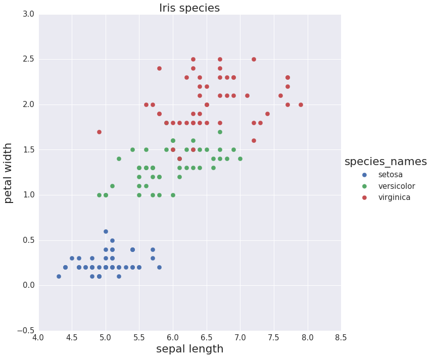
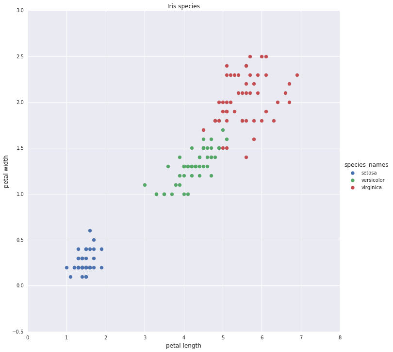
The Iris data set has four features (sepal length, sepal width, petal length, petal width) which can be used to classify Iris flowers into three species denoted as “0”, “1”, “2” (setosa, versicolor, virginica).
Scatter plot of Iris species
The K-nearest neighbors classifier is used to predict the species by using just two features: “sepal length” and “petal width”.
The graphs below show the predictions of the k-nearest neighbors algorithm using three different values for the number of nearest neighbors.
Using k-nearest neighbors to predict Iris species
When the k value is small (like the graph on the left) the decision boundary is relatively complex and even though the algorithm predicts the training data well, it is likely over-fitting the data and fair poorly on a new sample. For a very high value of k (like the graph on the right) the method the decision boundary is simpler and likely to under-fit the training data.
Random forests is an ensemble learning method. Ensemble methods use multiple learning algorithms to obtain better predictive performance than could be obtained for any of the constituent learning algorithms.
Random forests work by constructing multiple decision trees and combining the trees. The algorithm was developed by Leo Breiman and Adele Cutler and “Random Forests” is their trademark.
Random forests correct for decision trees’ habit of over-fitting to their training data set.
This Jupyter notebook contains all the code used to plot the charts.
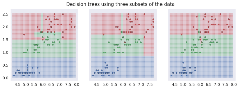
To demonstrate the tendency of decision trees to overfit the data we predict the species of Iris using just two features: sepal length and petal width. The species are shown in a scatter plot in different colors.
Scatter plot of Iris species
The graphs below show three Iris species using three different colors and the shaded regions predicted by the decision tree using lighter shades of the same colors. Each of the three plots in the set uses a different random sample made up of 70% of the data set. The decision tree boundaries are different in each case. This is an indication of over-fitting.
Using decision trees to predict Iris species
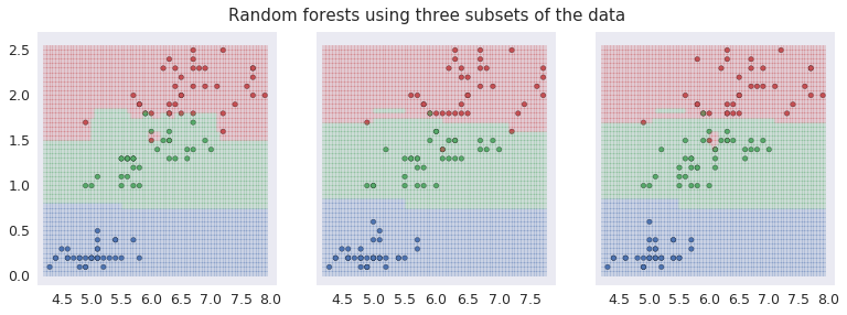
A similar plot shows a Random Forest Classifier with 500 trees each time used to select various sub-samples of the dataset. This controls over-fitting.
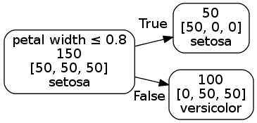
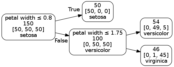
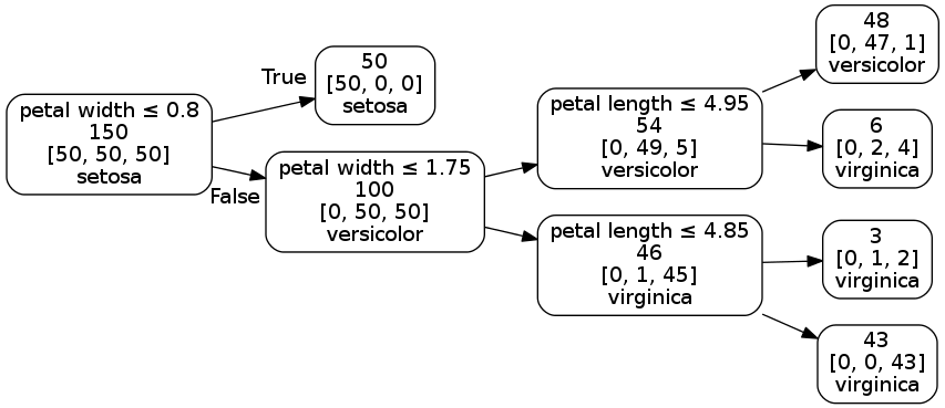
Decision trees are a non-parametric learning method used for classification and regression. Trees are often represented with a graph like model where each note is a test and each branch represents the outcome of the test.
We use the Iris data set to demonstrate the use of a decision tree classifier.
The Iris data set has four features (sepal length, sepal width, petal length, petal width) which can be used to classify Iris flowers into three species denoted as “0”, “1”, “2” (setosa, versicolor, virginica).
This Jupyter notebook contains all the code used to plot the charts.
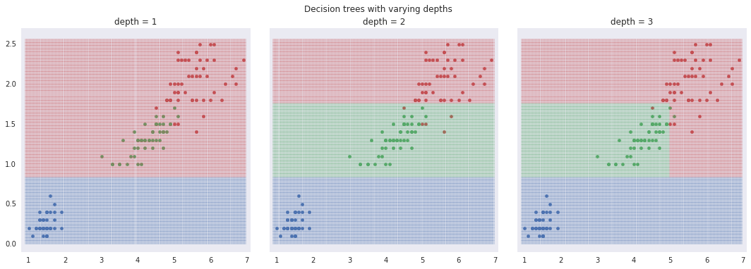
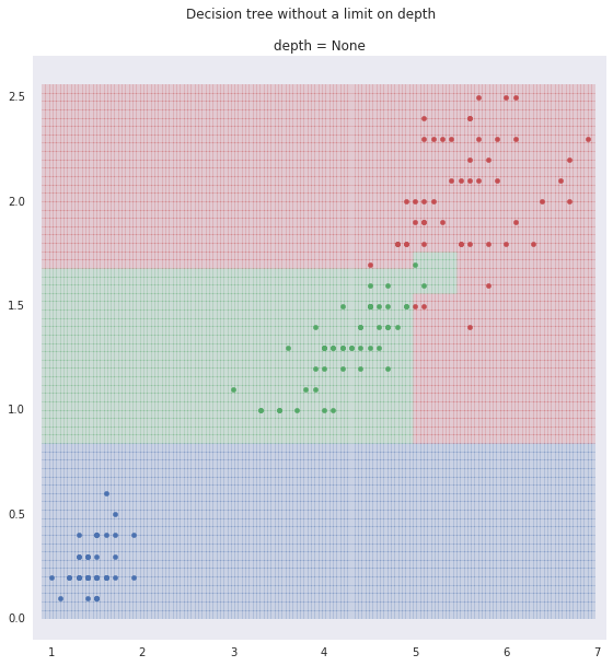
To better display the performance of the decision trees algorithm we predict
the species of Iris using just two features: petal length and petal width. The
species are shown in a scatter plot in different colors.
Scatter plot of Iris species
The output of the decision tree is shown using shaded regions that match the colors used to identify the flower. Using a decision tree with various depths the three species of Iris are classified, ineffectively at first with a tree of only one layer. As the number of layers increase the decision tree does a better job identifying the Iris species.
Decision trees classification boundaries
The decision tree rules can also be represented using a graph like drawing with the root node on the left and the leaf nodes on the right.
Finally we use a decision tree without limiting the depth. It classifies all the flowers correctly.
Support vector machines are supervised learning models used for
classification and regression. For a classifier the data is represented as
points in space and a SVM classifier (SVC) separates the classes by a gap that
is as wide as possible. SVM algorithms are known as maximum margin classifiers.
To illustrate the SVC algorithm we generate random points in two dimensions
arranged in two clusters. This is illustrated in a Jupyter (IPython) notebook
in this repository.
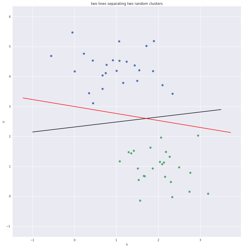
Multiple lines can be drawn to separate the clusters. The black line is
preferred to the red line as there is a larger margin between it and the
nearest points.
Some of the points nearest the boundary are known as support vectors. They
margins and the support vectors are plotted below.
Support vectors
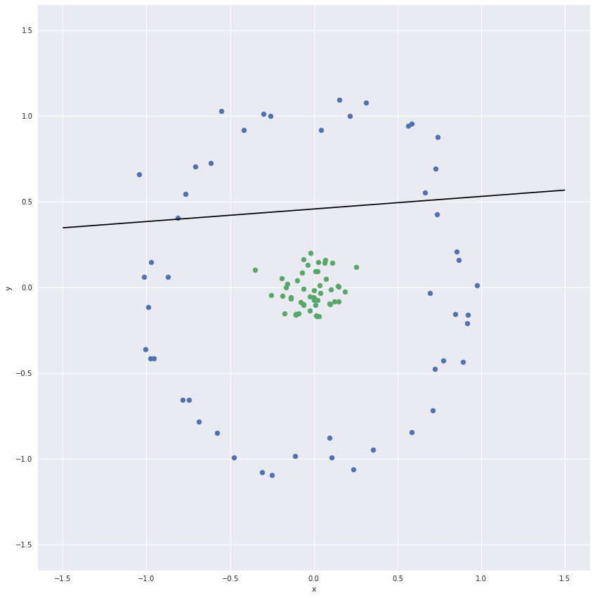
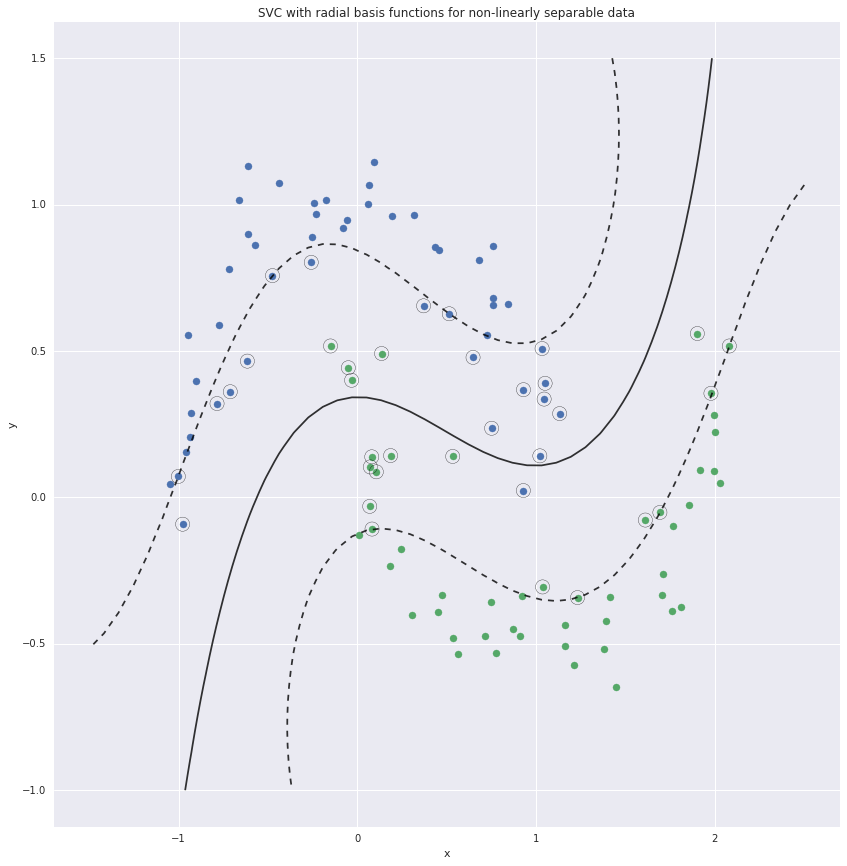
Support vector classifiers are linear classifiers. For datasets that are not
linearly separable they do a poor job.
Non-linearly separable data
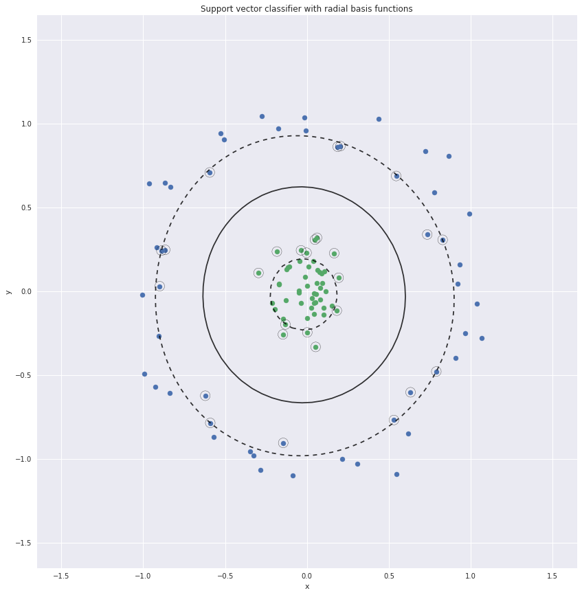
To create non-linear boundaries we could convert this two dimensional data set
to higher dimensions. For example we could add the distance of the points from
the origin as the third dimension. The two clusters will then be easily
separable.
The Iris data set has four features for Iris flower.
sepal length
sepal width
petal length
petal width
Using a three class logistic regression the four features can be used to
classify the flowers into three species (Iris setosa, Iris virginica,
Iris versicolor).
Using this Jupyter notebook combinations of two features we are used to
classify the species. The mis-predicted values are shown below.
measure 1
measure 2
incorrect predictions
sepal length
sepal width
29
sepal length
petal length
6
sepal length
petal width
8
sepal width
petal length
7
sepal width
petal width
7
petal length
petal width
6
The previous post shows that some combinations of
features are easier to use to separate the species than others.
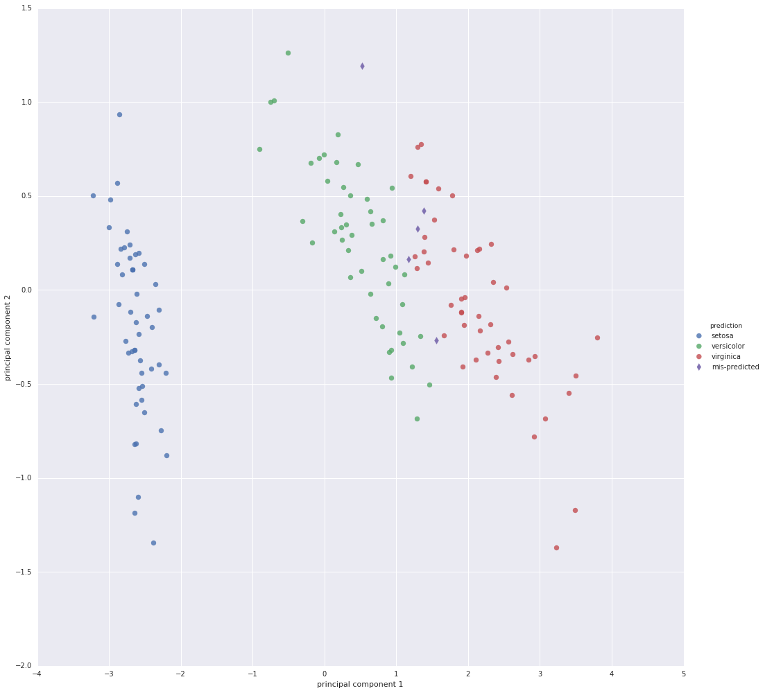
Logistic regression can also be used on the two principal components and
mis-predicts five specimens.
Iris plot with mis-predicted items
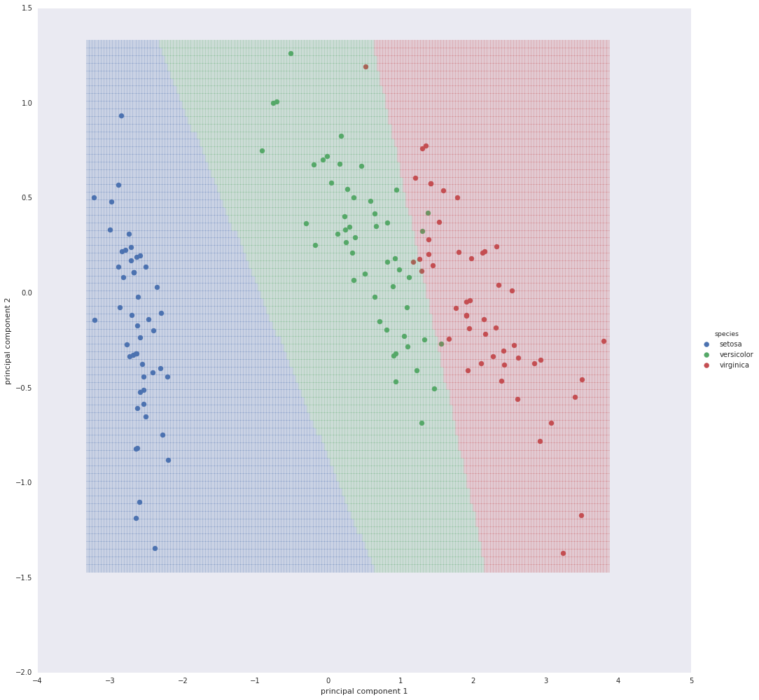
A mesh when drawn over the plot shows the three classes of the logistic
regression.
Scikit learn has multiple data sets included with the library. One of the most
well known data sets is the Iris data set introduced by Ronald Fisher.
Four features were measured from each sample: the length and the width of the
sepals and petals, in centimetres. Sepals are usually green and typically
function as protection for the flower in bud, and often as support for the
petals when in bloom. Based on the combination of these four features the
goal is to distinguish between three species of Iris
(Iris setosa, Iris virginica and Iris versicolor).
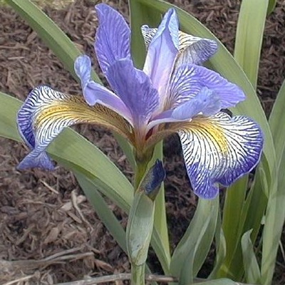
Iris setosa
Iris virginica
Iris versicolor
The data is shown in a Jupyter (IPython) notebook in this repository.
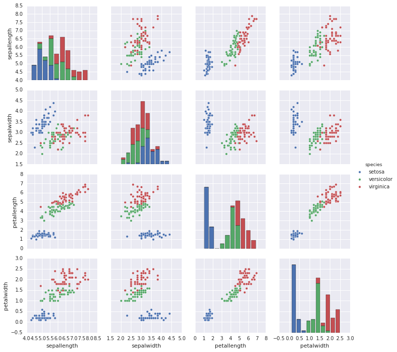
By converting the scikit-learn data into a pandas dataframe it can easily be
plotted using the seaborn library.
Seaborn iris plot
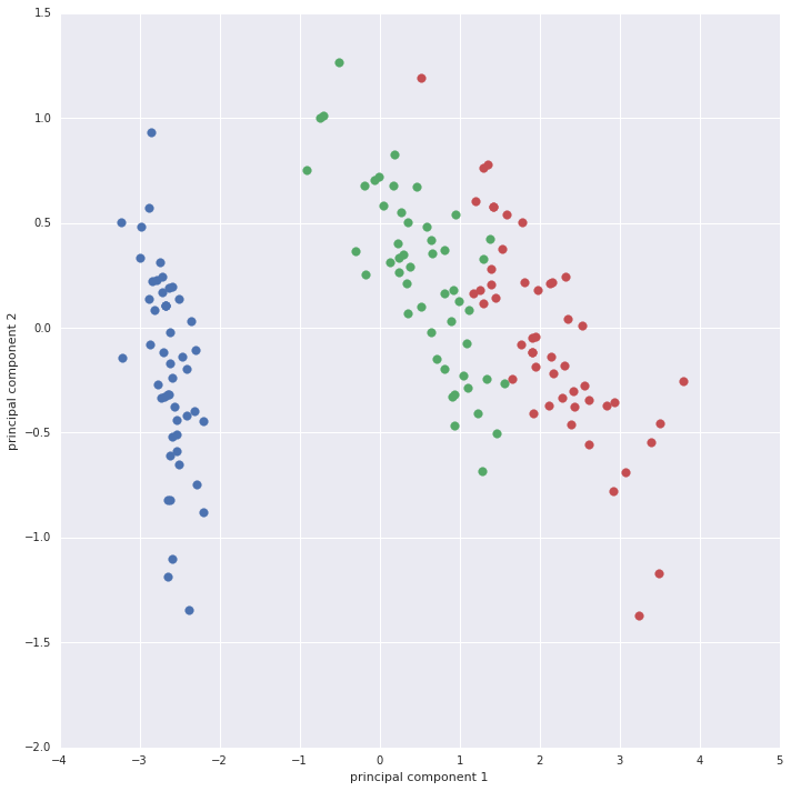
Using principal component analysis (PCA) the four dimensional data set can be
converted into a two dimensional data set by only choosing the first two
principal components.
This web site is created using Hugo a static web site generator.
Hyde Theme
Hyde is an elegant open source and mobile first theme for Hugo. Hyde a
two column theme that was ported from the theme of the same name made for
Jekyll another static web site generator writen in Ruby.
Making a post using Hugo
The content in Hugo is organized in sections. To make a new content file called
welcome.html in the section post run the following.
hugo new post/welcome.md
Adding images
To add an image to a markdown document you can use the following three options.